Dark energy

Conventions: We use $c=1$ for gravity and energy density $\rho$; section 3 restores $c$ in distances. Set $a_0=1$, so $1+z=1/a$. Dots mean cosmic-time derivatives. Distance examples assume spatial flatness. Dark energy names the component used to explain late cosmic acceleration within general relativity (GR); it does not identify a discovered particle.

1. Phenomenon: The Accelerating Universe

Why was acceleration surprising? Ordinary matter attracts and should slow an already expanding universe. The supernova teams found distant Type Ia supernovae dimmer, hence farther away after standardization, than decelerating reference models predicted. Their 1998 analysis and independent 1999 analysis inferred acceleration from the distance–redshift relation. They did not watch an individual galaxy gain speed in real time. Dust, source evolution and selection must be checked; agreement between different cosmological probes makes the explanation more persuasive.

The scale factor $a(t)$ describes distances between freely moving observers following the average cosmic flow. Homogeneity and isotropy give the FLRW metric below; $k$ encodes spatial curvature. Inserting a perfect-fluid stress tensor into Einstein's equations gives the two Friedmann equations. Here $\rho ,p$ exclude the separately written cosmological constant:

$$\begin{array}{c}d{s}^2=-d{t}^2+a^2(t)\left[\frac{d{r}^2}{1-k{r}^2}+r^{2}d{\Omega }^2\right],H=\frac{\dot{a}}{a}.\\ H^2=\frac{8\pi G}{3}\rho -\frac{k}{a^2}+\frac{\Lambda }{3},\frac{\ddot{a}}{a}=-\frac{4\pi G}{3}(\rho +3p)+\frac{\Lambda }{3}.\end{array}$$

Pressure gravitates in GR: the acceleration equation contains $\rho +3p$, not density alone. Positive density with sufficiently negative pressure can therefore accelerate expansion without being negative mass. Alternatively absorb $\Lambda$ into a fluid with ${\rho }_{\Lambda }=\Lambda /(8\pi G)$ and $p_{\Lambda }=-{\rho }_{\Lambda }$, and omit the explicit $\Lambda$ terms. Never count it twice. With positive total density, acceleration requires $w_{\mathrm{total}}=p_{\mathrm{total}}/{\rho }_{\mathrm{total}}<-1/3$. A small dark-energy component with $w<-1/3$ is insufficient if matter still dominates.

The deceleration parameter $q$ makes that distinction quantitative. The density fractions ${\Omega }_i$ are relative to $3H^2/(8\pi G)$ at the same epoch; the following expression treats dark energy as a fluid. An accelerating universe has $q<0$, but $H$ need not increase. Even when distances grow ever faster, their fractional growth rate can decrease.

$$q\equiv -\frac{\ddot{a}}{a{H}^2}=\frac{1}{2}{\Omega }_m+{\Omega }_r+\frac{1}{2}(1+3w){\Omega }_{\mathrm{DE}},\dot{H}=\frac{\ddot{a}}{a}-H^2.$$

Worked example: Take a flat matter-plus-$\Lambda$ model with ${\Omega }_{m0}=0.30$, ${\Omega }_{\Lambda 0}=0.70$ and negligible radiation, solely for illustration. Today $q_0=0.30/2-0.70=-0.55$. Since ${\rho }_m\propto a^{-3}$, acceleration starts at ${\rho }_m=2{\rho }_{\Lambda }$: $a_{\mathrm{acc}}=(0.30/1.40{)}^{1/3}\simeq 0.598$, or $z_{\mathrm{acc}}\simeq 0.67$. Equal matter and vacuum densities occur later, at $a\simeq 0.754$. Thus “dark energy exceeds matter” and “acceleration begins” are different thresholds.

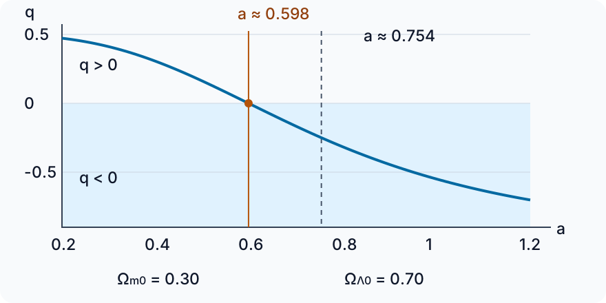
Acceleration has its own threshold. In the illustrative flat $({\Omega }_{m0},{\Omega }_{\Lambda 0})=(0.30,0.70)$ model, $q(a)$ crosses zero near $a=0.598$ (solid guide); density equality is near $a=0.754$ (dashed guide). The curve is calculated from the stated model, not fitted observations.

2. Equation of State and Parameterizations

Define $w=p_{\mathrm{DE}}/{\rho }_{\mathrm{DE}}$. For a homogeneous component exchanging no energy with other species, local stress-energy conservation gives the continuity equation. Dividing by $H\rho$ and using $d\ln a=Hdt$ produces an equation we can integrate:

$$\begin{array}{c}{\dot{\rho }}_{\mathrm{DE}}+3H({\rho }_{\mathrm{DE}}+p_{\mathrm{DE}})=0,\frac{d\ln {\rho }_{\mathrm{DE}}}{d\ln a}=-3(1+w).\\ {\rho }_{\mathrm{DE}}(a)={\rho }_{\mathrm{DE},0}\exp \left[-3{\int }_1^a(1+w(a^{\prime }))d\ln a^{\prime }\right].\end{array}$$

For constant $w$, this is $\rho \propto a^{-3(1+w)}$. Matter has $w\simeq 0$ and dilutes with volume; radiation has $w=1/3$, with an extra factor from photon redshift. A cosmological constant has $w=-1$ and constant density. The same result follows from $d(\rho V)=-pdV$ for a comoving volume $V\propto a^3$. Negative pressure lets its energy increase as the volume grows. This is consistent with local conservation; a generally expanding spacetime need not have a globally conserved total energy of the usual static-spacetime kind.

The Chevallier–Polarski–Linder (CPL) form compresses a possible time dependence into two parameters: the value today $w_0$ and a change coefficient $w_a$. Substituting it into the integral gives the density below; the exponential factor is essential. See the original Chevallier–Polarski and Linder papers.

$$\begin{array}{c}w(a)=w_0+w_a(1-a)=w_0+\frac{w_{a}z}{1+z},\\ \frac{{\rho }_{\mathrm{DE}}(z)}{{\rho }_{\mathrm{DE},0}}=(1+z{)}^{3(1+w_0+w_a)}\exp \left[-\frac{3w_{a}z}{1+z}\right].\end{array}$$

CPL is a fitting family, not a microscopic theory. It equals $\Lambda$ at $(w_0,w_a)=(-1,0)$ and may cross $w=-1$, which a single minimally coupled canonical scalar with positive energy cannot do. For $w<-1$, a positive-density perfect fluid has $\rho +p<0$ and violates the null energy condition; an effective fit need not imply a fundamental ghost field. CPL also diverges as $a\to \infty$ when $w_a\ne 0$, so extrapolating it to the remote future is unjustified.

3. Background Observables

Telescopes measure fluxes, angles, spectra and correlations. A model converts them to distances and expansion rates; no instrument reads a dark-energy density directly. Each probe supplies a different piece of that conversion.

3.1 Hubble Expansion

Define ${\Omega }_{i0}={\rho }_{i0}/{\rho }_{c0}$, with ${\rho }_{c0}=3H_0^2/(8\pi G)$. In a flat universe the fractions sum to one. Separately conserved matter, radiation and dark energy give:

$$\frac{H^2(z)}{H_0^2}={\Omega }_{r0}(1+z{)}^4+{\Omega }_{m0}(1+z{)}^3+{\Omega }_{\mathrm{DE},0}\frac{{\rho }_{\mathrm{DE}}(z)}{{\rho }_{\mathrm{DE},0}}.$$

At $z=1$ in the example above, $H/H_0=\sqrt{0.30\times 8+0.70}\simeq 1.761$. Replace $w=-1$ by constant $w=-0.8$, keeping today's fractions and $H_0$ fixed: the dark-energy term becomes $0.70\times 2^{0.6}$ and $H/H_0\simeq 1.860$. Dark-energy density at this redshift changes by about 52%, but the total expansion rate changes by only 5.7%. Matter dilutes the effect, and integrated distances smooth it further. This illustrates why measuring time variation is demanding.

3.2 Distances (SNe Ia, BAO, CMB)

For a radial light ray, $d{s}^2=0$ relates distance to the integral of $1/H$. In flat space the comoving distance $\chi$, luminosity distance $d_L$ and angular-diameter distance $D_A$ are related as follows. Curvature replaces $\chi$ by a curvature-dependent transverse distance in the last two relations. The usual distance duality also assumes photons follow null geodesics and their number is conserved.

$$\begin{array}{c}\chi (z)=c{\int }_0^z\frac{d{z}^{\prime }}{H(z^{\prime })},d_L=(1+z)\chi ,D_A=\frac{\chi }{1+z},\\ \mu =5{\log }_{10}\left(\frac{d_L}{10\mathrm{pc}}\right),D_V={\left[(1+z{)}^2{D}_A^2\frac{cz}{H(z)}\right]}^{1/3}.\end{array}$$

A source of calibrated luminosity $L$ and flux $F$ obeys $F=L/(4\pi d_L^2)$. SNe Ia are standardizable, not perfectly identical candles: light-curve shape, color and host corrections matter. The modulus $\mu$ logarithmically packages the distance. An uncalibrated supernova sample mostly measures relative distances; absolute luminosity and $H_0$ are degenerate. A 0.10-magnitude shift changes inferred distance by $10^{0.10/5}-1\simeq 4.7\%$, illustrating the importance of calibration.

Baryon acoustic oscillations (BAO) use a statistical preferred separation imprinted by early plasma sound waves. The comoving sound horizon $r_d$ is evaluated at the baryon drag epoch. Across the line of sight BAO constrain $D_M/r_d$; along it they constrain $D_H/r_d$, with $D_H=c/H$. The schematic small-separation relations are:

$${\theta }_{\mathrm{BAO}}\simeq \frac{r_d}{D_M(z)},\Delta z_{\mathrm{BAO}}\simeq \frac{H(z)r_d}{c},D_M=(1+z)D_A.$$

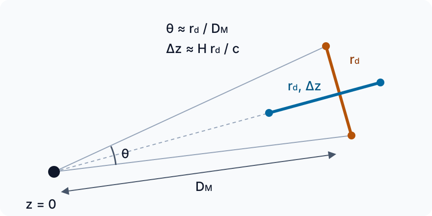
One statistical ruler, two directions. The orange transverse separation relates $r_d$ to angle $\theta$ and $D_M$; the blue radial separation relates $r_d$ to $\Delta z$ and $H$. Geometry is schematic, and the ruler is comoving.

The cube-averaged distance $D_V$ summarizes an isotropic BAO analysis; anisotropic analyses retain radial and transverse information. BAO are a correlation feature, not rigid rods carried by individual galaxies. The CMB constrains early densities and acoustic scales and helps calibrate $r_d$. Inferring late-time parameters still assumes a model of the early universe: changing early expansion can change the ruler. The Planck parameter analysis is a concrete example of these conditional inferences.

4. Growth of Structure

Expansion is only half the test. Matter overdensities $\delta =\delta {\rho }_m/{\rho }_m$ also grow through attraction. For linear, subhorizon, pressureless matter perturbations in GR, with smooth dark energy and negligible radiation contributions, continuity, Euler and Poisson equations combine to give:

$$\ddot{\delta }+2H\dot{\delta }-4\pi G{\rho }_m\delta =0,f\equiv \frac{d\ln D}{d\ln a}.$$

Here $\delta \propto D(a)$ describes the growing mode. The $2H\dot{\delta }$ term damps growth, while the density term drives it. In a flat matter-only era $D\propto a$; once smooth dark energy matters, growth slows relative to $a$. The approximation $f\simeq {\Omega }_m(a{)}^{0.55}$ is useful near $\Lambda$CDM, not an identity valid for every model or scale. Redshift-space distortions constrain combinations such as $f{\sigma }_8$; ${\sigma }_8$ is the rms linear density contrast in spheres of radius $8h^{-1}$ Mpc, with $h=H_0/(100\mathrm{km}{\mathrm{s}}^{-1}\mathrm{Mp}{\mathrm{c}}^{-1})$.

Galaxy motions respond to the Newtonian potential $\Psi$, while lensing probes a combination $\Phi +\Psi$. Using the Fourier convention ${\nabla }^2\to -k^2$, one often parameterizes departures from a reference model as:

$$k^2\Psi =-4\pi G_{\mathrm{eff}}(k,a)a^2{\rho }_m\Delta ,\eta =\frac{\Phi }{\Psi }.$$

Here $\Delta$ is the comoving matter-density perturbation; this $k$ is a wavenumber, not the background curvature symbol. In GR with negligible anisotropic stress, $G_{\mathrm{eff}}=G$ and $\eta =1$. Neutrino stress or other imperfect components can also produce gravitational slip in GR. A measured discrepancy therefore requires checking matter physics, galaxy bias and observational systematics before attributing it to modified gravity.

5. Microscopic Models (Sketch)

A background fit for $w$ does not uniquely identify a field or gravity theory. Models that share $H(z)$ may have different perturbations, stability conditions and local-gravity behavior.

5.1 Cosmological Constant $\Lambda$

A Lorentz-invariant vacuum has a stress tensor proportional to the metric. Its pressure is negative even though its energy density can be positive:

$$T_{\mu \nu }^{(\Lambda )}=-{\rho }_{\Lambda }{g}_{\mu \nu },p_{\Lambda }=-{\rho }_{\Lambda },{\rho }_{\Lambda }=\frac{\Lambda }{8\pi G}.$$

The cosmological-constant problem is why the renormalized total vacuum contribution, including the gravitational constant term and quantum corrections, is so small. A cutoff estimate is not a measured prediction: its numerical mismatch depends on the assumed energy scale and regularization. Merely adding a free $\Lambda$ fits the observed value but does not explain its stability against large corrections. This conceptual issue remains even if observations ultimately select $w=-1$; see Peebles and Ratra's theoretical discussion.

The coincidence question is distinct: why do we observe an epoch when matter and vacuum densities are comparable, although their ratio changes as $a^3$? It motivates dynamical proposals but is not evidence that such proposals are true.

5.2 Quintessence

Quintessence models introduce a canonical, minimally coupled scalar field. For a homogeneous field with metric signature $(-,+,+,+)$, kinetic energy $K$ and potential $V$ give:

$$\begin{array}{c}\mathcal{L}=-\frac{1}{2}{g}^{\mu \nu }{\partial }_{\mu }\varphi {\partial }_{\nu }\varphi -V(\varphi ),\\ K=\frac{1}{2}{\dot{\varphi }}^2,{\rho }_{\varphi }=K+V,p_{\varphi }=K-V,w_{\varphi }=\frac{K-V}{K+V}.\end{array}$$

Varying the action gives the field equation; it also follows by inserting ${\rho }_{\varphi },p_{\varphi }$ into the continuity equation where $\dot{\varphi }\ne 0$. The $3H\dot{\varphi }$ term acts as cosmological friction.

$$\ddot{\varphi }+3H\dot{\varphi }+V_{,\varphi }=0,{\rho }_{\varphi }+3p_{\varphi }=4K-2V.$$

If this field dominates, acceleration requires $K<V/2$. When $K\ll V$, it resembles a cosmological constant; when $V=0$, it has $w=1$, so a scalar does not automatically accelerate the universe. For $K,V\ge 0$ and positive density, $-1\le w\le 1$. Inverse-power or exponential potentials can admit tracking behavior for suitable parameters, reducing sensitivity to some initial conditions without eliminating tuning. Their potential, couplings and perturbative stability remain physical assumptions, not consequences of a successful CPL fit.

5.3 Modified Gravity (MG)

Modified gravity changes the relation between matter and curvature. Metric $f(R)$ theories, for example, generally introduce an extra scalar degree of freedom. Chameleon screening can suppress its local effects; Vainshtein screening occurs in other derivative-interaction theories. Neither is a universal property of all models. Horndeski and degenerate higher-order scalar-tensor theories organize broader possibilities. GW170817 and its gamma-ray counterpart tightly constrain the relative propagation speed of gravity and light in the observed regime, excluding many proposed interactions under their assumptions; they do not eliminate all modified gravity.

6. Tensions and Consistency Checks

The Hubble tension compares early-universe, model-dependent $H_0$ inference with local distance-ladder determinations. The Planck analysis illustrates the former; it is not a direct local expansion measurement. Changing late dark energy is not automatically a solution, because the same change must fit BAO and supernova distances. “Early dark energy” is a separate proposal affecting an earlier epoch, not simply another name for today's accelerating component.

Similarly, $S_8={\sigma }_8\sqrt{{\Omega }_m/0.3}$ summarizes an important lensing degeneracy, not all information in a lensing survey. Differences between growth and CMB inference depend on the dataset, nonlinear modeling, baryonic feedback, redshift calibration and intrinsic galaxy alignments. It is better to compare full likelihoods and shared nuisance parameters than to treat every apparent tension as independent evidence for new physics.

7. Inference Pipeline (Practical Notes)

1. Specify the model and priors: curvature, neutrino masses, early physics and whether dark energy clusters; $w_0,w_a$ alone are not a full theory.
2. Compute $H$, distances, early acoustic scales and linear perturbations consistently. Precision work uses a Boltzmann solver, not only a growth-index fit or a compressed CMB distance prior.
3. Predict measured statistics with selection, calibration and nuisance parameters. Retain covariance between overlapping datasets; multiplying correlated likelihoods as though independent double-counts information.
4. Sample the posterior and test goodness of fit, prior dependence and leave-one-probe-out stability. More parameters can improve a fit without establishing a new physical component.

8. Status

Evidence checked through 13 October 2026. The 2025 DESI DR2 BAO paper found BAO alone well described by flat $\Lambda$CDM. In the CPL extension, BAO+CMB favored evolving dark energy at $3.1\sigma$; adding different supernova compilations gave $2.8$–$4.2\sigma$. These are specified comparisons with $(w_0,w_a)=(-1,0)$, not a direct detection of a scalar field.

The 2026 full DES multi-probe analysis, combining geometry and growth, reported a $2.2\sigma$ deviation within CPL for DES alone, $2.3\sigma$ after adding DESI DR2 BAO, and $3.0\sigma$ with primary CMB information. Those combinations overlap other analyses; their significances must not be multiplied as independent confirmations.

The July 2026 DESI Lyα full-shape analysis, revised in August, added an Alcock–Paczyński geometry measurement at effective redshift $2.33$. The new anchor moved toward $\Lambda$CDM; the paper reports a $2.7\sigma$ CPL preference with DESI+CMB and $3.2\sigma$ when also including its supernova dataset. Thus the evidence is evolving and sensitive to which information enters the fit.

A quoted number of standard deviations is conditional on the model, likelihood and systematic-error treatment; it is not the probability that dark energy evolves. The open questions are whether independent calibration and growth tests preserve the pattern, which physical theory could produce it stably, and whether a simpler explanation survives. Current hints deserve investigation, while the microscopic origin of acceleration remains unresolved.

Common misconceptions: Dark energy is not the dark matter that clusters in halos. Negative pressure does not mean negative energy density or a wind pushing galaxies from a central point. Bound atoms, solar systems and galaxies do not simply follow the cosmological scale factor. Finally, neither an accelerating present nor a finite-redshift CPL fit determines the universe's ultimate fate: a constant vacuum, a changing potential and a future instability have different extrapolations.